Natural language feels effortless to humans. We read sentences, infer emotions, detect intent, and understand context almost instantly. For machines, however, language is far from intuitive. It is symbolic, ambiguous, and fundamentally unstructured. 

So how do we teach machines to understand text? 

The answer lies in embeddings—a foundational idea that quietly powers almost every modern NLP system today. Their importance becomes even more evident in small language models (SLMs), where efficiency, compactness, and meaningful representations matter far more than sheer scale. 

This blog walks through how embeddings evolved, why they replaced traditional text representations, and how they form the backbone of resource-efficient NLP systems. 

Why Text Needs to Become Numbers

Computers do not understand words the way humans do—they understand numbers.

A sentence like “Machine learning is fascinating” carries meaning for us, but to a machine, it is merely a sequence of characters. Before any learning can happen, this text must be transformed into a numerical form. This process is known as text representation, and the quality of this representation directly affects how well a model can learn patterns, relationships, and meaning from data. 

Before Embeddings: Traditional Text Representation Techniques 

Before embeddings became the norm, NLP systems relied on explicit, rule-based methods to convert text into numbers. These approaches were simple and interpretable, but they struggled to capture semantic meaning. 

Let’s look at them more closely. 

One-Hot Encoding 

One-hot encoding represents each word as a vector whose length equals the vocabulary size. In this vector, exactly one position is set to 1, while all others are 0. Each word is uniquely identified, but no information about meaning or similarity is preserved. 

For example, consider the sentence: 

“I love NLP” 

With a vocabulary of ["I", "love", "NLP"], each word is mapped to a unique vector. While this representation is easy to understand, it treats every word as equally distant from every other word. There is no notion of similarity—“love” is no closer to “like” than it is to “banana”. 

This approach quickly becomes impractical for real-world NLP due to its high dimensionality, sparsity, and inability to generalize beyond seen words. As a result, one-hot encoding is mostly limited to toy examples and theoretical explanations. 

Bag of Words (BoW) 

Bag of Words improves upon one-hot encoding by representing an entire document as a vector of word counts. Instead of encoding individual words, it counts how frequently each word appears in a document, ignoring word order, grammar, and context. 

For instance, the sentences “NLP is fun” and “Fun is NLP” produce identical representations under BoW, even though word order has changed. While BoW captures frequency information, it still fails to encode meaning. Common words and rare but informative words are treated equally, and semantic relationships remain invisible. 

TF-IDF (Term Frequency–Inverse Document Frequency) 

TF-IDF was introduced to address one of BoW’s biggest shortcomings: overemphasizing common words. Words like “is”, “the”, or “and” appear frequently but contribute little meaning. 

TF-IDF balances this by combining: 

• Term Frequency (TF), which measures how often a word appears in a document 

• Inverse Document Frequency (IDF), which penalizes words that appear across many documents 

As a result, words that are frequent in a specific document but rare across the corpus receive higher importance. TF-IDF is more informative than BoW and works well for tasks like document classification and information retrieval.  However, TF-IDF still treats words as independent symbols. It cannot understand context, semantic similarity, or synonyms—“happy” and “joyful” remain unrelated. 

Why Traditional Methods Fell Short 

Despite incremental improvements, traditional text representations share a fundamental limitation: they treat words as isolated tokens rather than carriers of meaning. They cannot capture semantics, understand similarity, or generalize well across contexts.

This gap is precisely what led to the rise of embeddings. 

The Birth of Embeddings: A Paradigm Shift 

Embeddings introduced a powerful idea: represent words as dense vectors where distance encodes meaning. 

Instead of sparse vectors with thousands of dimensions, embeddings use compact, continuous vectors—often between 50 and 300 dimensions—that are learned directly from data. In this space, semantically similar words naturally cluster together. “King” lies closer to “queen” than to “apple”, and “Paris” is closer to “France” than to “dog”.

This single shift fundamentally changed how machines process language. 

Dimensionality of Embeddings: How Big Should Meaning Be? 

One important design choice when working with embeddings is deciding their dimensionality—that is, how many numbers are used to represent each word. 

Lower-dimensional embeddings (e.g., 50 dimensions): 

• Use less memory 

• Train faster 

• May miss subtle semantic details  

Higher-dimensional embeddings (e.g., 300 dimensions):

• Capture richer relationships 

• Require more data and memory 

• Risk overfitting in small datasets 

In practice, small language models often favor moderate dimensions (50–200), striking a balance between expressiveness and efficiency. More dimensions do not automatically mean better understanding—what matters is how well those dimensions capture useful patterns. 

Mathematical Intuition Behind Embeddings 

Embeddings map words into a continuous vector space. Within this space, relationships become geometric. Meaning is encoded through direction and distance rather than discrete identifiers. 

A classic example illustrates this idea: 

vector("king") - vector("man") + vector("woman") ≈ vector("queen") 

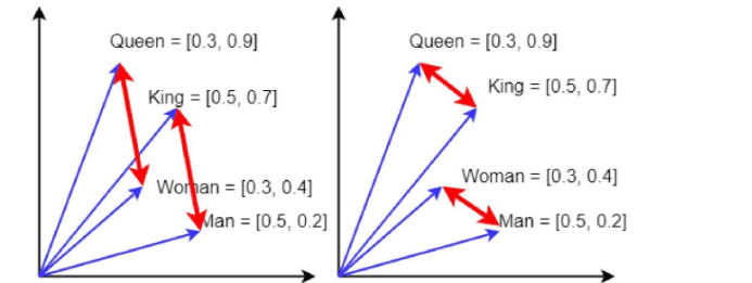
Similarity between words is often measured using cosine similarity, which focuses on the angle between vectors rather than their magnitude—making it well suited for semantic comparison. 

Measuring Similarity in Embedding Space 

Once words are represented as vectors, understanding meaning becomes a question of distance. 

Two commonly used distance measures are Euclidean distance and cosine similarity. 

Euclidean distance measures straight-line distance between two vectors. While intuitive, it can be sensitive to vector magnitude and is less commonly used for semantic comparison. 

Cosine similarity, on the other hand, measures the angle between two vectors. It focuses on direction rather than magnitude, making it far more suitable for embeddings. 

That is why cosine similarity is the default choice in tasks like:

• Semantic search 

• Word similarity 

• Recommendation systems 

In embedding space, words with similar meanings point in similar directions—even if their vector lengths differ. 

Latent Factors 

A natural question that arises is: What does each dimension of an embedding represent? 

The answer is—there is no simple answer. 

Embedding dimensions are latent factors, meaning they do not correspond to explicit human-defined features. A single dimension might partially encode multiple ideas such as gender, tense, topic, or sentiment. Individually, these dimensions are difficult to interpret, but together they form a rich representation of meaning. 

This is why embeddings are best understood geometrically rather than symbolically. Instead of asking what a specific dimension means, it is more useful to observe how words relate to one another through distance and direction. 

Types of Embeddings in NLP 

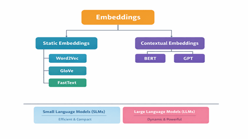
Static Word Embeddings 

Static embeddings assign exactly one vector to each word, regardless of context. They are based on the distributional hypothesis: words that appear in similar contexts tend to have similar meanings. 

Word2Vec 

One of the most important turning points in Natural Language Processing came with the introduction of Word2Vec. Until then, machines could count words, but they couldn’t truly understand them. Word2Vec changed that by showing that meaning doesn’t come from a word alone—it comes from how that word is used. 

At its heart, Word2Vec is based on a simple idea we intuitively follow as humans: 

You understand a word by the company it keeps. 

If two words regularly appear in similar surroundings, chances are they share a related meaning. Word2Vec learns this pattern directly from raw text, without any manual labeling or linguistic rules. 

How Word2Vec Learns Meaning  

Word2Vec does not try to memorize dictionary definitions. Instead, it looks at large amounts of text and learns which words tend to appear together. Over time, it builds a mathematical space where related words naturally move closer to each other. 

Technically, Word2Vec is implemented as a very shallow neural network with just one hidden layer. During training, words are first represented as one-hot vectors, passed through the network, and adjusted based on prediction errors. Once training is complete, the network itself is discarded—only the learned vectors remain. 

Those vectors are the embeddings. They are dense, compact, and surprisingly expressive. 

Embedding Matrix: Where Word Meanings Are Stored 

When Word2Vec finishes training, it doesn’t store meanings as rules or probabilities. Instead, it stores everything inside a structure called the embedding matrix. 

The embedding matrix is essentially a table where:

• Each row corresponds to a word 

• Each row vector is that word’s embedding 
   

If your vocabulary has V words and each embedding has D dimensions, the embedding matrix has a shape: 

(V × D) 

For example, a vocabulary of 10,000 words with 100-dimensional embeddings results in a 10,000 × 100 matrix. 

This matrix acts as a lookup table. Whenever a word appears, the model simply fetches its corresponding vector. In small language models, this matrix often contains the majority of the model’s learned knowledge, making it one of the most important components. 

The Distributional Hypothesis in Action 

Word2Vec relies on the distributional hypothesis, which states that words occurring in similar contexts tend to have similar meanings. 

For example:

• king, queen, and prince frequently appear near words related to royalty 

• cat and dog appear near words associated with pets 

• Paris and France often appear in geographic contexts 

By learning from these patterns, Word2Vec creates embeddings where semantic relationships emerge naturally—without being explicitly programmed. 

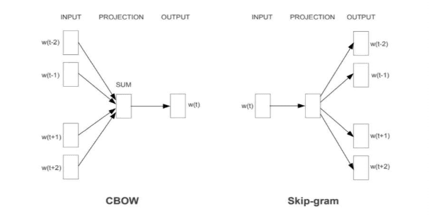
Two Ways Word2Vec Learns: CBOW and Skip-Gram 

Word2Vec can be trained using two slightly different strategies. Both lead to meaningful embeddings, but they approach learning from opposite directions. 

CBOW (Continuous Bag of Words) 

CBOW tries to predict a missing word using the words around it. 

Consider the sentence:

I like deep learning 

With a small context window, the model might see the words “I” and “deep” and learn to predict the word “like”. Over many such examples, CBOW learns which words tend to complete similar contexts. 

CBOW is generally fast and efficient. It works especially well when trained on large datasets and tends to perform well for frequently occurring words. However, because it averages context information, it can sometimes lose subtle semantic details. 

Skip-Gram 

Skip-Gram flips the problem around. Instead of predicting the center word, it predicts the surrounding words given a target word. 

Using the same sentence: 

I like deep learning 

The model takes “like” as input and learns to predict nearby words such as “I” and “deep”. This approach forces the model to learn richer representations, especially for words that do not appear very often. 

Skip-Gram usually trains more slowly than CBOW, but it produces higher-quality embeddings for rare words and smaller datasets. Because of this, it is often the preferred choice in practice. 

Word2Vec Code Example- 

Below is a minimal example using the gensim library to train a Word2Vec model. 

from gensim.models import Word2Vec 

# Sample corpus 

sentences = [ 

    ["i", "love", "nlp"], 

    ["nlp", "is", "interesting"], 

    ["i", "love", "machine", "learning"], 

    ["deep", "learning", "is", "powerful"] 

] 

# Train the Word2Vec model 

model = Word2Vec( 

    sentences=sentences, 

    vector_size=50,

    window=3, 

    min_count=1, 

    sg=1  # sg=1 → Skip-Gram, sg=0 → CBOW 

) 

# Access the embedding for a word 

print(model.wv["nlp"]) 

Finding Similar Words 

model.wv.most_similar("learning", topn=3) 

This returns words that are closest to “learning” in the embedding space. 

Measuring Semantic Similarity 

similarity = model.wv.similarity("nlp", "learning") 

print(similarity) 

Higher values indicate stronger semantic similarity. 

Negative Sampling 

Training Word2Vec naïvely would be computationally expensive. For every word, the model would need to consider the entire vocabulary—a task that quickly becomes infeasible for large datasets. 

Negative sampling solves this problem elegantly. 

Instead of comparing a word against every possible alternative, the model focuses on a small number of examples. It treats real word–context pairs as positive examples and randomly samples a few unrelated words as negative examples. The model then learns to distinguish between what should appear together and what should not. 

This approach dramatically reduces computation while still producing high-quality embeddings. For small language models, negative sampling is one of the key reasons Word2Vec remains both effective and efficient. 

GloVe 

Word2Vec learns meaning by observing local context windows, adjusting word vectors based on nearby words. While this works well, it raises an important question: is local context enough to fully capture meaning? 

GloVe (Global Vectors for Word Representation) answers this by looking at the entire corpus at once. Instead of predicting words like Word2Vec, GloVe builds a global word co-occurrence matrix that records how often words appear together across the dataset. 

The key idea behind GloVe is simple yet powerful: 
word meaning is encoded in the ratios of co-occurrence probabilities. 

For instance, words like ice and steam relate differently to cold and hot. These relationships become clear only when viewed globally, not through isolated windows. By factorizing the co-occurrence matrix, GloVe learns dense vectors that capture both semantic similarity and linear relationships, which is why analogies like: 

king − man + woman ≈ queen 

work so well. 

Compared to Word2Vec, GloVe benefits from global statistical consistency and a more interpretable training objective. However, it still assigns one fixed vector per word, meaning multiple meanings of a word (like bank) are merged into a single representation. Additionally, storing large co-occurrence matrices can be memory-heavy for very large vocabularies. 

FastText 

Word2Vec and GloVe treat words as indivisible units. FastText challenges this assumption by recognizing that words have internal structure, and that structure carries meaning. 

FastText breaks words into character n-grams. For example, the word learning is represented using smaller units like lea, ear, arn, and ing. Instead of learning one vector per word, FastText learns vectors for these subword components and combines them. 

This allows FastText to:

• Handle rare and unseen words 

• Understand morphology (tense, plurality, prefixes) 

• Remain robust to misspellings and noisy text 

As a result, FastText performs especially well for morphologically rich languages and low-resource datasets. The trade-off is slightly higher computational cost and larger model size compared to Word2Vec and GloVe. 

Word2Vec vs GloVe vs FastText 

Closing Thought 

Word2Vec showed that meaning emerges from context. 
GloVe proved that global statistics refine meaning. 
FastText revealed that words themselves carry structure. 

Together, these static embeddings laid the groundwork for modern NLP and remain highly valuable—especially for small language models, where efficiency, compactness, and strong prior knowledge are essential. 

Where Small Language Models Fit In 

As language models grew more capable, a natural assumption emerged: bigger is always better. More parameters, more data, more computation—surely that must lead to better understanding. And in many cases, it does. 

But reality tells a more nuanced story. 

Not every system needs billions of parameters to function well. Many real-world applications—mobile apps, embedded systems, enterprise tools, and domain-specific products—operate under tight constraints. Limited memory, limited compute, and limited latency budgets make massive models impractical. This is where Small Language Models (SLMs) quietly shine. 

SLMs are designed with efficiency in mind. They focus on doing just enough—learning strong representations without the overhead of massive architectures. And in this setting, how words are represented becomes far more important than how large the model is. 

Why Static Embeddings Are a Natural Fit for SLMs 

Static word embeddings such as Word2Vec, GloVe, and FastText align almost perfectly with the philosophy of small language models. 

These embeddings act like compressed knowledge capsules. Long before the model begins training, they already encode semantic relationships, syntactic patterns, and distributional meaning. When an SLM uses these embeddings, it does not have to rediscover language structure from scratch—it inherits it. 

Because static embeddings: 

• Are lightweight 

• Require no dynamic computation per sentence 

• And have a fixed memory footprint 

They allow SLMs to remain fast, predictable, and efficient. 

In many NLP pipelines, static embeddings serve as a strong foundation layer, enabling small models to punch far above their weight. For tasks like text classification, sentiment analysis, search, and recommendation, this combination often delivers surprisingly strong performance. 

The Trade-Off: What SLMs Gain and What They Miss 

Small Language Models offer several clear advantages: 

They are faster to train and deploy, easier to debug, and far more economical in terms of memory and compute. Their behavior is more stable and predictable, which makes them ideal for production environments with strict constraints. 

However, this efficiency comes with limitations. 

SLMs struggle when meaning depends heavily on context. A static embedding assigns one meaning per word, regardless of how that word is used. As a result, sentences that rely on nuance, ambiguity, or long-range dependencies can be difficult to interpret correctly. 

This is where Large Language Models (LLMs) step in. 

LLMs compensate for these limitations by learning context dynamically. Instead of relying on a single vector per word, they generate representations that change based on surrounding words, sentence structure, and even broader discourse. The cost is high—massive models, long training times, and significant compute requirements—but the payoff is a far deeper understanding of language. 

In short: 

• SLMs trade depth for efficiency 

• LLMs trade efficiency for depth 

Both exist because both are needed. 

Contextual Embeddings: A Brief Look Ahead 

Static embeddings laid the foundation, but contextual embeddings represent the next chapter. 

In contextual models, a word does not have a single fixed meaning. Instead, its representation shifts with context. The word bank becomes one vector near river and a completely different one near money. This dynamic understanding is at the heart of transformer-based LLMs like BERT and GPT. 

Rather than replacing static embeddings entirely, contextual embeddings build upon their ideas—learning richer, more flexible representations at scale. 

Closing the Loop 

The story of embeddings is not about replacing old ideas with new ones. It is about choosing the right tool for the right problem. 

Static embeddings power efficient, reliable systems where resources matter. 
Small language models bring focus and practicality. 
Large language models push the boundaries of understanding. 

Together, they form a continuum—one where meaning is not just learned, but engineered with intent.